Table of contents:

• A visual representation
• Optimization for Machine Learning: Gradient Descent
• Cost Function for Linear Regression
• What are its strengths and weaknesses

Linear regression is used to predict real-valued outputs, and it assumes a linear dependence/ relationship between the variables of the dataset. Hence, it is a parametric algorithm. In linear regression, the prevailing assumption is that the output or the response variable (i.e., the unit that we want to predict) can be modeled as a linear combination of the input (or predictor) variables. A linear combination is the addition of a certain number of vectors scaled (or adjusted) by an arbitrary constant. A vector is a mathematical construct for representing a set of numbers.

Figure 1: Dataset with real-valued outputs

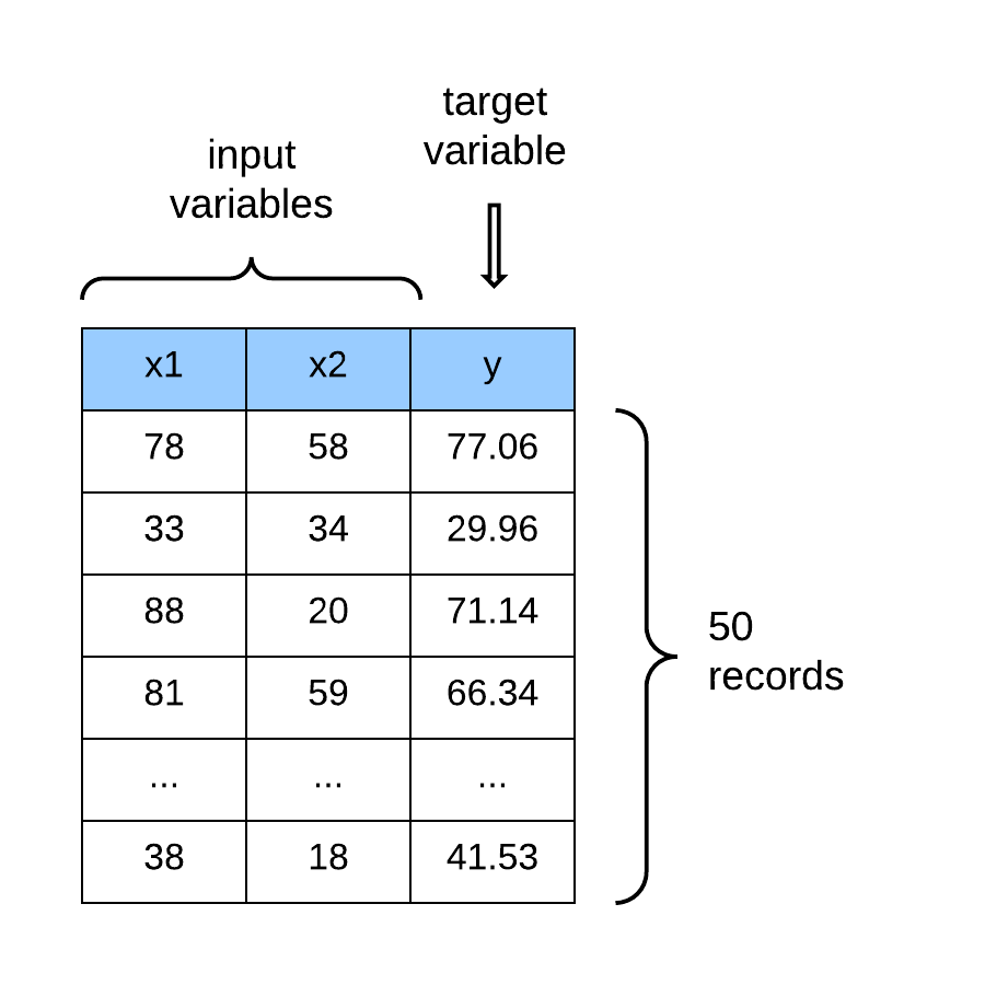
In a linear regression model, every variable (or feature vector) is assigned a specific weight (or parameter). We say that a weight parameterizes each feature in the dataset. The weights (or parameters) in the dataset are adjusted to find the optimal value (or constant) that scales the features to optimally approximate the values of the target (or output variable). The linear regression model is formally represented as:

$$\hat{y}=θ_0+θ_1 x_1+θ_2 x_2+...+θ_n x_n$$

A visual representation

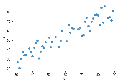
To illustrate, the image below is a plot of the first feature and the target variable . We are plotting just one feature against the output variable because it is easier to visualize using a 2-D scatter plot.

Figure 2: Scatter plot of x and y

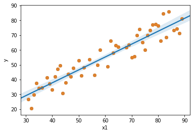
So the goal of the linear model is to find a line that gives the best approximation or the best fit to the data points. When found, that line will look like the blue line in the image below.

Figure 3: Scatter plot with the regression line

Optimization for Machine Learning: Gradient Descent

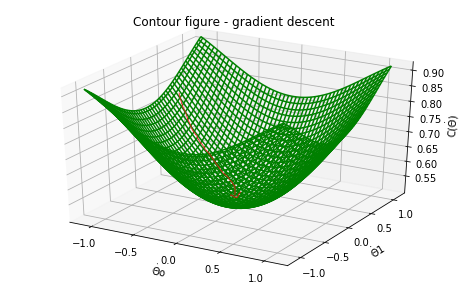
Gradient descent is an optimization algorithm that is used to minimize a function (in this case we will be decreasing the cost or loss function of an algorithm). A cost function in machine learning is a measure that you want to minimize. We can also see the cost as the penalty you pay for having a bad or incorrect model approximation.

Gradient descent attempts to find an approximate solution or the global minimum of the function space by moving iteratively in step along the path of steepest descent until a terminating condition is reached that stops the loop or the algorithm converges.

Figure 4: Gradient Descent

Cost Function for Linear Regression

In the case of the linear regression model, the cost function is defined as half the sum of the squared difference between the predicted value and the actual value. The linear regression cost function is formally called the squared-error cost function and is represented as:

$$C(θ)=\frac{1}{2} \sum (\hat{y}-y)^2$$

To put it more simply, the closer the approximate value of the target variable is to the actual variable, the lower our cost and the better our model. Now that we have defined the cost function that we want to minimize, we use gradient descent to minimize the cost. In the wild, a variety of names are used to represent linear regression such as ordinary least squares or least squares regression.

What are its strengths and weaknesses

Linear regression is hard to beat as the algorithm of choice when the fundamental structure of the learning problem is linear. Moreso, it even surprisingly performs reasonably well on non-linear datasets.

However, the more exciting learning problems in practice have variables with complex non-linear relationships. Linear regression becomes infeasible as an algorithm of choice for building a prediction model. Even when we have lots of data which mitigates the presence of high-dimensional datasets, linear regression is still bound to perform poorly in light of more sophisticated non-linear machine learning techniques.