Working with Keras on GCP Notebook Instance
Source Code and Contribution:
The entire source code is available on Github at: https://github.com/dvdbisong/Working-with-Keras
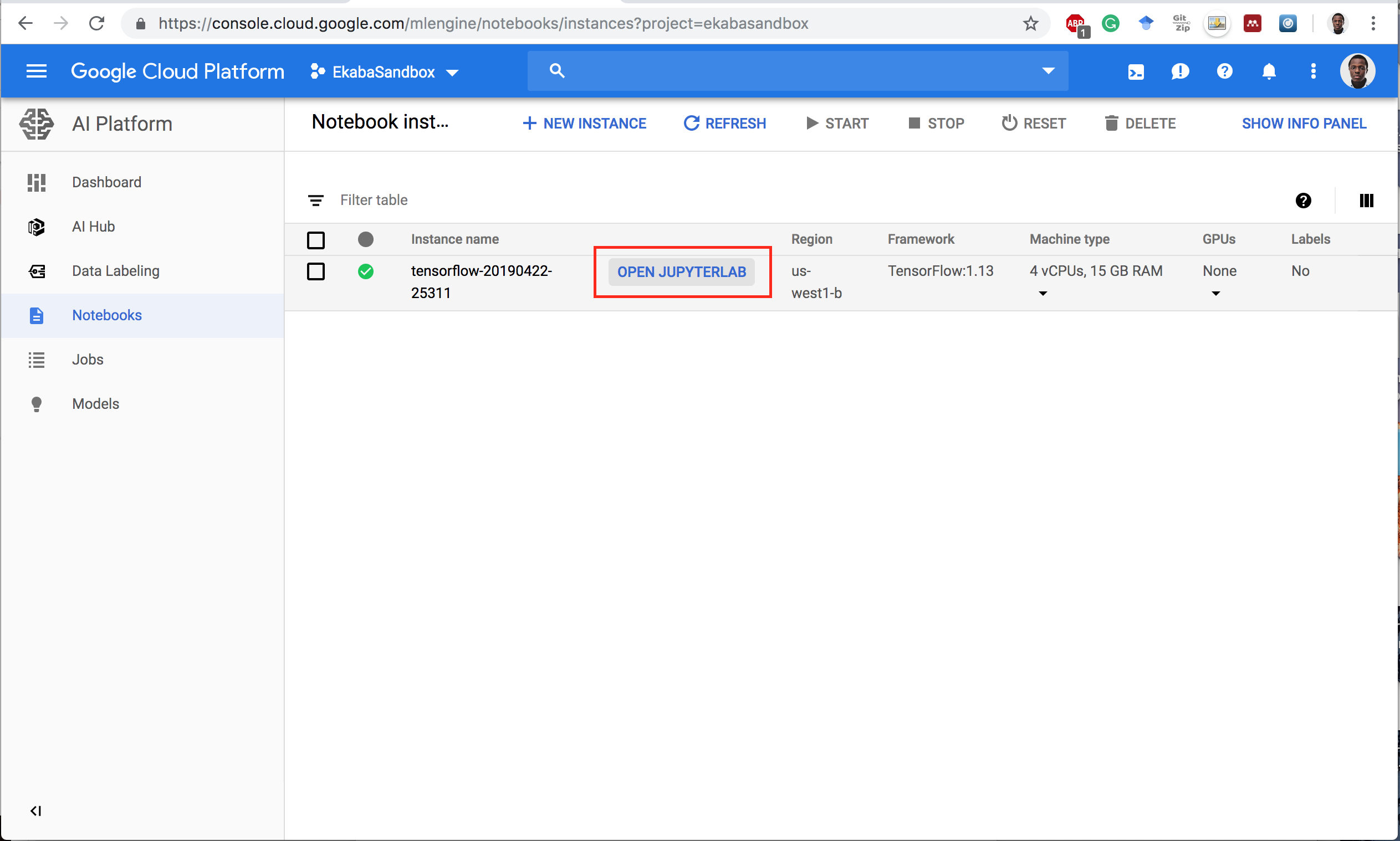
Notebook Instance on GCP AI Platform
Open Notebook Instance

Notebook Instances Dashboard

Start a New Instance


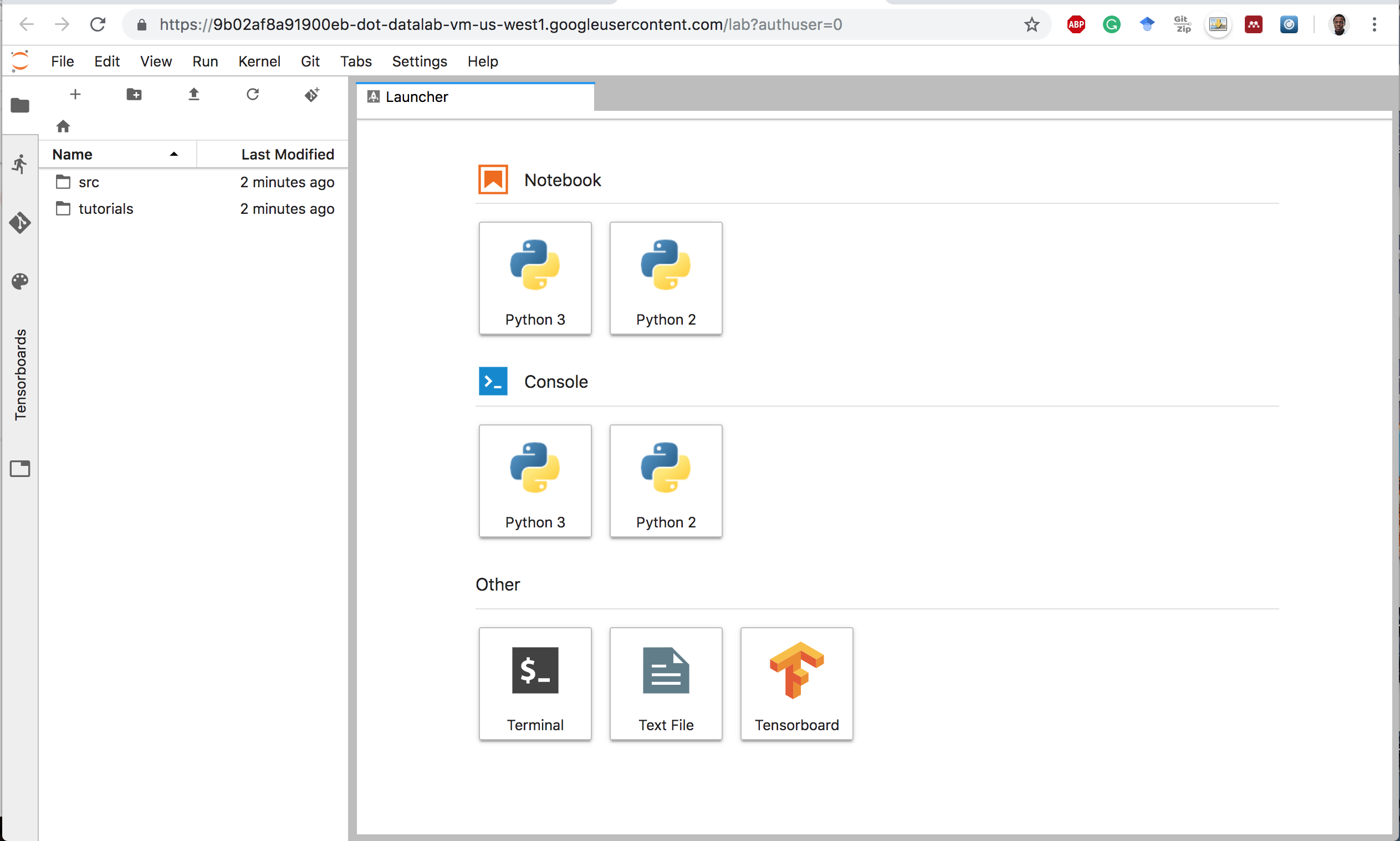
Open Jupyterlab
The Anatomy of a Keras Program
- The Keras Model is the core of a Keras programme.
- A Model is:
- constructed,
- compiled, then
- trained and evaluated using their respective training and evaluation datasets.
- Upon satisfactory evaluation, the model is used to make predictions on previously unseen data.
Program flow for modeling with Keras.
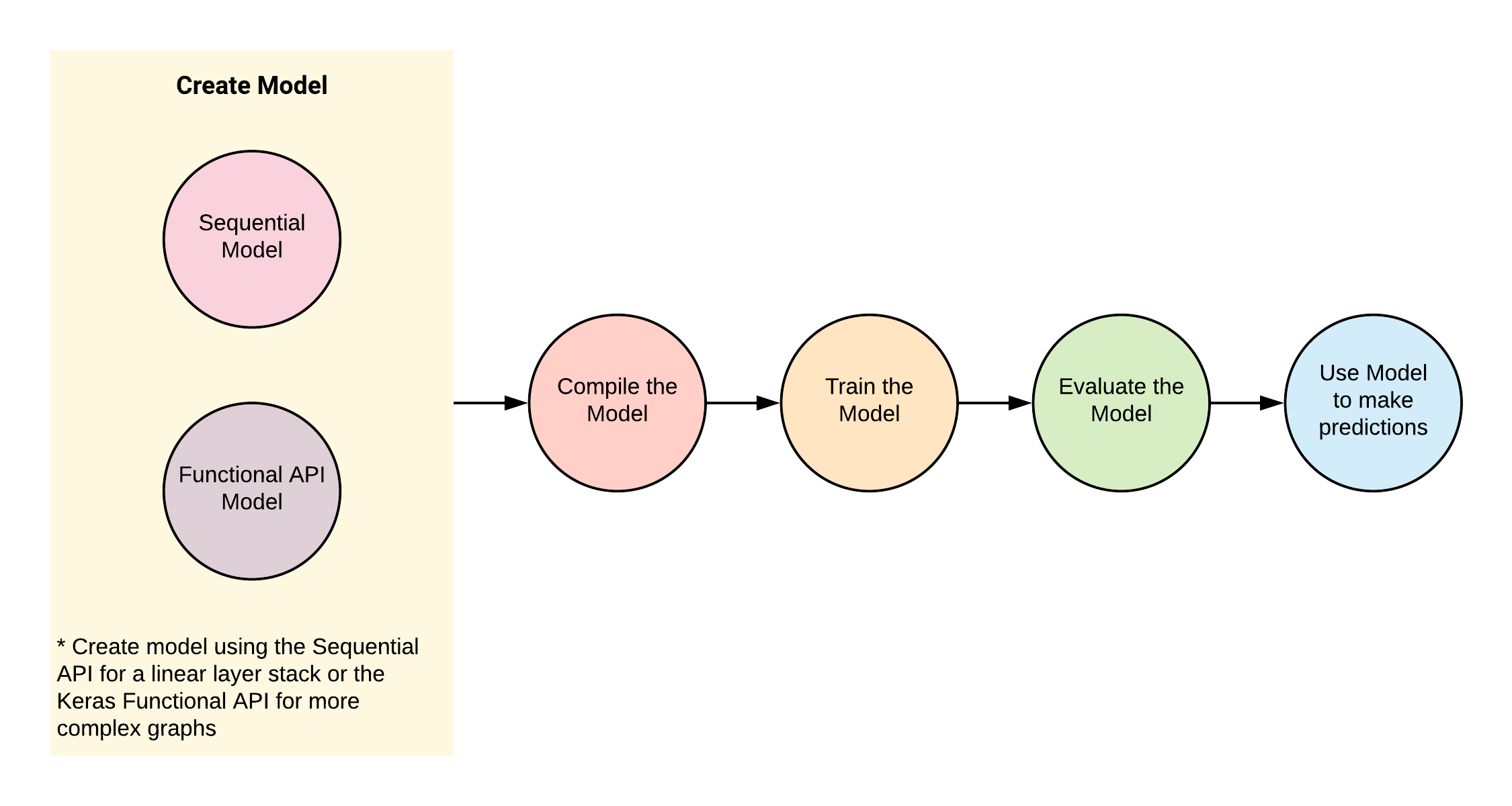
The Keras API
A Keras Model can be constructed using:
- The Sequential API
tf.keras.Sequential(simple API for creating a linear stack of Neural Networks layers), or - The Keras Functional API which defines a model instance
tf.keras.Modelfor more complex network graphs.
Multilayer Perceptron (MLP) with Keras
We'll go through the following steps:
- Import and transform the dataset.
- Build and Compile the Model
- Train the data using
Model.fit() - Evaluate the Model using
Model.evaluate() - Predict on unseen data using
Model.predict()
The Dataset
- The dataset used for this example is the Fashion-MNIST database of fashion articles.
- It is similar to the MNIST handwriting dataset.
- It contains 60,000 28x28 pixel grayscale images.
This dataset and more can be found in the
tf.keras.datasetspackage.
Preprocess
Flatten from 2-dimensional shape to 1-dimension
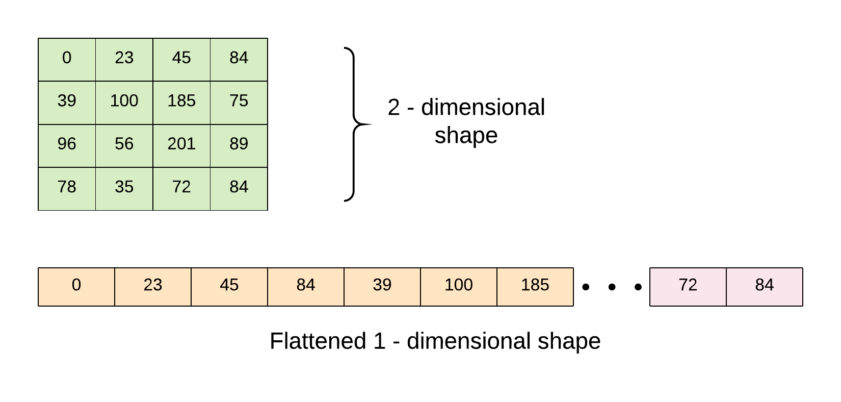
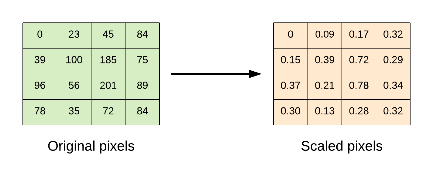
Scale pixels from 0 to 255 to be within the range of 0 to 1.
Code
pythonimport tensorflow as tf import numpy as np # import dataset (x_train, y_train), (x_test, y_test) = tf.keras.datasets.fashion_mnist.load_data() # flatten the 28*28 pixel images into one long 784 pixel vector x_train = np.reshape(x_train, (-1, 784)).astype('float32') x_test = np.reshape(x_test, (-1, 784)).astype('float32') # scale dataset from 0 -> 255 to 0 -> 1 x_train /= 255 x_test /= 255 # one-hot encode targets y_train = tf.keras.utils.to_categorical(y_train) y_test = tf.keras.utils.to_categorical(y_test) # create the model def model_fn(): model = tf.keras.Sequential() # Adds a densely-connected layer with 256 units to the model: model.add(tf.keras.layers.Dense(256, activation='relu', input_dim=784)) # Add Dropout layer model.add(tf.keras.layers.Dropout(0.2)) # Add another densely-connected layer with 64 units: model.add(tf.keras.layers.Dense(64, activation='relu')) # Add a softmax layer with 10 output units: model.add(tf.keras.layers.Dense(10, activation='softmax')) # compile the model model.compile(optimizer=tf.train.AdamOptimizer(0.001), loss='categorical_crossentropy', metrics=['accuracy']) return model # build model model = model_fn() # train the model model.fit(x_train, y_train, epochs=10, batch_size=100, verbose=1, validation_data=(x_test, y_test)) # evaluate the model score = model.evaluate(x_test, y_test, batch_size=100) print('Test loss: {:.2f} \nTest accuracy: {:.2f}%'.format(score[0], score[1]*100))
Using the Dataset API with tf.keras
- The Dataset API is the preferred mechanism for feeding data as it can easily scale to handle very large datasets and better utilize the machine resources.
- The data pipeline is constructed using the Dataset API and the Model is constructed using the Keras Functional API.
Code
pythonimport tensorflow as tf import numpy as np # import dataset (x_train, y_train), (x_test, y_test) = tf.keras.datasets.fashion_mnist.load_data() # flatten the 28*28 pixel images into one long 784 pixel vector x_train = np.reshape(x_train, (-1, 784)).astype('float32') x_test = np.reshape(x_test, (-1, 784)).astype('float32') # scale dataset from 0 -> 255 to 0 -> 1 x_train /= 255 x_test /= 255 # one-hot encode targets y_train = tf.keras.utils.to_categorical(y_train) y_test = tf.keras.utils.to_categorical(y_test) # create dataset pipeline def input_fn(features, labels, batch_size, training=True): dataset = tf.data.Dataset.from_tensor_slices((features, labels)) if training: dataset = dataset.shuffle(buffer_size=1000) dataset = dataset.repeat() dataset = dataset.batch(batch_size) iterator = dataset.make_one_shot_iterator() features, labels = iterator.get_next() return features, labels # parameters batch_size = 100 training_steps_per_epoch = int(np.ceil(x_train.shape[0] / float(batch_size))) # ==> 600 eval_steps_per_epoch = int(np.ceil(x_test.shape[0] / float(batch_size))) # ==> 100 epochs = 10 # create the model def model_fn(input_fn): (features, labels) = input_fn # Model input model_input = tf.keras.layers.Input(tensor=features) # Adds a densely-connected layer with 256 units to the model: x = tf.keras.layers.Dense(256, activation='relu', input_dim=784)(model_input) # Add Dropout layer: x = tf.keras.layers.Dropout(0.2)(x) # Add another densely-connected layer with 64 units: x = tf.keras.layers.Dense(64, activation='relu')(x) # Add a softmax layer with 10 output units: predictions = tf.keras.layers.Dense(10, activation='softmax')(x) # the model model = tf.keras.Model(inputs=model_input, outputs=predictions) # compile the model model.compile(optimizer='adam', loss='categorical_crossentropy', metrics=['accuracy'], target_tensors=[tf.cast(labels,tf.float32)]) return model # build train model model = model_fn(input_fn(x_train, y_train, batch_size=batch_size, training=True)) # print train model summary model.summary()
python# train the model history = model.fit(epochs=epochs, steps_per_epoch=training_steps_per_epoch)
python# store trained model weights model.save_weights('/tmp/mlp_weight.h5') # build evaluation model eval_model = model_fn(input_fn(x_test, y_test, batch_size=batch_size, training=False)) # load saved weights to evaluation model eval_model.load_weights('/tmp/mlp_weight.h5') # evaluate the model score = eval_model.evaluate(steps=eval_steps_per_epoch) print('Test loss: {:.2f} \nTest accuracy: {:.2f}%'.format(score[0], score[1]*100))
TensorBoard with Keras
To visualize models with TensorBoard, attach a TensorBoard callback tf.keras.callbacks.TensorBoard() to the model.fit() method before training the model. The model graph, scalars, histograms, and other metrics are stored as event files in the log directory.
For this example, we'll build an MLP MNIST model and visualize it with TensorBoard.
Code
pythonimport tensorflow as tf import numpy as np # import dataset (x_train, y_train), (x_test, y_test) = tf.keras.datasets.mnist.load_data() # flatten the 28*28 pixel images into one long 784 pixel vector x_train = np.reshape(x_train, (-1, 784)).astype('float32') x_test = np.reshape(x_test, (-1, 784)).astype('float32') # scale dataset from 0 -> 255 to 0 -> 1 x_train /= 255 x_test /= 255 # one-hot encode targets y_train = tf.keras.utils.to_categorical(y_train) y_test = tf.keras.utils.to_categorical(y_test) # create the model def model_fn(): inputs = tf.keras.Input(shape=(784,)) x = tf.keras.layers.Dense(128, activation='relu', input_dim=784)(inputs) x = tf.keras.layers.Dropout(0.2)(x) x = tf.keras.layers.Dense(64, activation='relu')(x) prediction = tf.keras.layers.Dense(10, activation='softmax')(x) model = tf.keras.Model(inputs=inputs, outputs=prediction) # compile the model model.compile(optimizer='adam', loss='categorical_crossentropy', metrics=['accuracy']) return model # build model model = model_fn() # checkpointing best_model = tf.keras.callbacks.ModelCheckpoint('./tmp/mnist_weights.h5', monitor='val_acc', verbose=1, save_best_only=True, mode='max') # tensorboard tensorboard = tf.keras.callbacks.TensorBoard(log_dir='./tmp/logs_mnist_keras', histogram_freq=0, write_graph=True, write_images=True) callbacks = [best_model, tensorboard] # train the model history = model.fit(x_train, y_train, epochs=10, batch_size=100, verbose=1, validation_data=(x_test, y_test), callbacks=callbacks) # evaluate the model score = model.evaluate(x_test, y_test, batch_size=100) print('Test loss: {:.2f} \nTest accuracy: {:.2f}%'.format(score[0], score[1]*100))
python# execute the command to run TensorBoard.
python!tensorboard --logdir tmp/logs_mnist_keras
Checkpointing to Select Best Models
- Checkpointing makes it possible to save the weights of the neural network model when there is an increase in the validation accuracy metric.
- This is achieved in Keras using the method
tf.keras.callbacks.ModelCheckpoint(). - The saved weights can then be loaded back into the model and used to make predictions.
Using the MNIST dataset, we'll build a model that saves the weights to file only when there is an improvement in the validation set performance.
Code
pythonimport tensorflow as tf import numpy as np # import dataset (x_train, y_train), (x_test, y_test) = tf.keras.datasets.mnist.load_data() # flatten the 28*28 pixel images into one long 784 pixel vector x_train = np.reshape(x_train, (-1, 784)).astype('float32') x_test = np.reshape(x_test, (-1, 784)).astype('float32') # scale dataset from 0 -> 255 to 0 -> 1 x_train /= 255 x_test /= 255 # one-hot encode targets y_train = tf.keras.utils.to_categorical(y_train) y_test = tf.keras.utils.to_categorical(y_test) # create the model def model_fn(): inputs = tf.keras.Input(shape=(784,)) x = tf.keras.layers.Dense(128, activation='relu', input_dim=784)(inputs) x = tf.keras.layers.Dropout(0.2)(x) x = tf.keras.layers.Dense(64, activation='relu')(x) prediction = tf.keras.layers.Dense(10, activation='softmax')(x) model = tf.keras.Model(inputs=inputs, outputs=prediction) # compile the model model.compile(optimizer='adam', loss='categorical_crossentropy', metrics=['accuracy']) return model # build model model = model_fn() # checkpointing checkpoint = tf.keras.callbacks.ModelCheckpoint('mnist_weights.h5', monitor='val_acc', verbose=1, save_best_only=True, mode='max') callbacks = [checkpoint] # train the model history = model.fit(x_train, y_train, epochs=10, batch_size=100, verbose=1, validation_data=(x_test, y_test), callbacks=callbacks) # evaluate the model score = model.evaluate(x_test, y_test, batch_size=100) print('Test loss: {:.2f} \nTest accuracy: {:.2f}%'.format(score[0], score[1]*100))
Convolutional Neural Networks (CNNs) with Keras
In this section, we use Keras to implement a Convolutional Neural Network. The network architecture is similar to the Krizhevsky architecture and consists of the following layers:
- Convolution layer: kernel_size => [5 x 5]
- Convolution layer: kernel_size => [5 x 5]
- Batch Normalization layer
- Convolution layer: kernel_size => [5 x 5]
- Max pooling: pool size => [2 x 2]
- Convolution layer: kernel_size => [5 x 5]
- Convolution layer: kernel_size => [5 x 5]
- Batch Normalization layer
- Max pooling: pool size => [2 x 2]
- Convolution layer: kernel_size => [5 x 5]
- Convolution layer: kernel_size => [5 x 5]
- Convolution layer: kernel_size => [5 x 5]
- Max pooling: pool size => [2 x 2]
- Dropout layer
- Dense Layer: units => [512]
- Dense Layer: units => [256]
- Dropout layer
- Dense Layer: units => [10]
Dataset
- The dataset used for this example is the Cifar10 image dataset.
- It consists of 60000 32x32 colour images in 10 classes, with 6000 images per class.
- There are 50000 training images and 10000 test images.
- The 10 classes are: [airplane, automobile, bird, cat, deer, dog, frog, horse, ship, truck]
This dataset and more can be found in the tf.keras.datasets package.
Code
python# import dataset (x_train, y_train), (x_test, y_test) = tf.keras.datasets.cifar10.load_data() # change datatype to float x_train = x_train.astype('float32') x_test = x_test.astype('float32') # scale the dataset from 0 -> 255 to 0 -> 1 x_train /= 255 x_test /= 255 # one-hot encode targets y_train = tf.keras.utils.to_categorical(y_train) y_test = tf.keras.utils.to_categorical(y_test) # create dataset pipeline def input_fn(features, labels, batch_size, training=True): dataset = tf.data.Dataset.from_tensor_slices((features, labels)) if training: dataset = dataset.shuffle(buffer_size=1000) dataset = dataset.repeat() dataset = dataset.batch(batch_size) iterator = dataset.make_one_shot_iterator() features, labels = iterator.get_next() return features, labels # parameters batch_size = 100 training_steps_per_epoch = int(np.ceil(x_train.shape[0] / float(batch_size))) # ==> 600 eval_steps_per_epoch = int(np.ceil(x_test.shape[0] / float(batch_size))) # ==> 100 epochs = 10 # create the model def model_fn(input_fn): (features, labels) = input_fn # Model input model_input = tf.keras.layers.Input(tensor=features) x = tf.keras.layers.Conv2D(64, (5, 5), padding='same', activation='relu')(model_input) x = tf.keras.layers.Conv2D(64, (5, 5), padding='same', activation='relu')(x) x = tf.keras.layers.BatchNormalization()(x) x = tf.keras.layers.Conv2D(64, (5, 5), padding='same', activation='relu')(x) x = tf.keras.layers.MaxPooling2D(pool_size=(2, 2), strides=2, padding='same')(x) x = tf.keras.layers.Conv2D(64, (5, 5), padding='same', activation='relu')(x) x = tf.keras.layers.Conv2D(64, (5, 5), padding='same', activation='relu')(x) x = tf.keras.layers.BatchNormalization()(x) x = tf.keras.layers.MaxPooling2D(pool_size=(2, 2), strides=2, padding='same')(x) x = tf.keras.layers.Conv2D(32, (3, 3), padding='same', activation='relu')(x) x = tf.keras.layers.Conv2D(32, (3, 3), padding='same', activation='relu')(x) x = tf.keras.layers.Conv2D(32, (3, 3), padding='same', activation='relu')(x) x = tf.keras.layers.MaxPooling2D(pool_size=(2, 2), strides=2, padding='same')(x) x = tf.keras.layers.Dropout(0.3)(x) x = tf.keras.layers.Flatten()(x) x = tf.keras.layers.Dense(512, activation='relu')(x) x = tf.keras.layers.Dense(256, activation='relu')(x) x = tf.keras.layers.Dropout(0.5)(x) output = tf.keras.layers.Dense(10, activation='softmax')(x) # the model model = tf.keras.Model(inputs=model_input, outputs=output) # compile the model model.compile(optimizer=tf.keras.optimizers.Nadam(), loss='categorical_crossentropy', metrics=['accuracy'], target_tensors=[tf.cast(labels,tf.float32)]) return model # build train model model = model_fn(input_fn(x_train, y_train, batch_size=batch_size, training=True)) # print train model summary model.summary()
python# train the model history = model.fit(epochs=epochs, steps_per_epoch=training_steps_per_epoch)
python# store trained model weights model.save_weights('./tmp/cnn_weight.h5') # build evaluation model eval_model = model_fn(input_fn(x_test, y_test, batch_size=batch_size, training=False)) eval_model.load_weights('./tmp/cnn_weight.h5') # evaluate the model score = eval_model.evaluate(steps=eval_steps_per_epoch) print('Test loss: {:.2f} \nTest accuracy: {:.2f}%'.format(score[0], score[1]*100))
Recurrent Neural Networks (RNNs) with Keras
This section uses the Nigeria power consumption univariate timeseries dataset to implement a LSTM Recurrent Neural Network.
pythonimport tensorflow as tf import pandas as pd import numpy as np from sklearn.model_selection import train_test_split from sklearn.preprocessing import MinMaxScaler # data url url = "https://raw.githubusercontent.com/dvdbisong/gcp-learningmodels-book/master/Chapter_12/nigeria-power-consumption.csv" # load data parse_date = lambda dates: pd.datetime.strptime(dates, '%d-%m') data = pd.read_csv(url, parse_dates=['Month'], index_col='Month', date_parser=parse_date, engine='python', skipfooter=2) # print column name data.columns # change column names data.rename(columns={'Nigeria power consumption': 'power-consumption'}, inplace=True) # split in training and evaluation set data_train, data_eval = train_test_split(data, test_size=0.2, shuffle=False) # MinMaxScaler - center ans scale the dataset scaler = MinMaxScaler(feature_range=(0, 1)) data_train = scaler.fit_transform(data_train) data_eval = scaler.fit_transform(data_eval) # adjust univariate data for timeseries prediction def convert_to_sequences(data, sequence, is_target=False): temp_df = [] for i in range(len(data) - sequence): if is_target: temp_df.append(data[(i+1): (i+1) + sequence]) else: temp_df.append(data[i: i + sequence]) return np.array(temp_df) # parameters time_steps = 20 inputs = 1 neurons = 100 outputs = 1 batch_size = 32 # create training and testing data train_x = convert_to_sequences(data_train, time_steps, is_target=False) train_y = convert_to_sequences(data_train, time_steps, is_target=True) eval_x = convert_to_sequences(data_eval, time_steps, is_target=False) eval_y = convert_to_sequences(data_eval, time_steps, is_target=True) # Build model model = tf.keras.Sequential() model.add(tf.keras.layers.LSTM(128, dropout=0.2, recurrent_dropout=0.2, input_shape=train_x.shape[1:], return_sequences=True)) model.add(tf.keras.layers.Dense(1)) # Compile the model model.compile(loss='mean_squared_error', optimizer='adam', metrics=['mse']) # print model summary model.summary()
python# Train the model history = model.fit(train_x, train_y, batch_size=batch_size, epochs=20, shuffle=False, validation_data=(eval_x, eval_y))
pythonloss, mse = model.evaluate(eval_x, eval_y, batch_size=batch_size) print('Test loss: {:.4f}'.format(loss)) print('Test mse: {:.4f}'.format(mse)) # predict y_pred = model.predict(eval_x) # plot predicted sequence plt.title("Model Testing", fontsize=12) plt.plot(eval_x[0,:,0], "b--", markersize=10, label="training instance") plt.plot(eval_y[0,:,0], "g--", markersize=10, label="targets") plt.plot(y_pred[0,:,0], "r--", markersize=10, label="model prediction") plt.legend(loc="upper left") plt.xlabel("Time")